
#Keras 基础
参考文档
#安装
# 安装 Tensorflow
pip install tensorflow --user -i https://pypi.tuna.tsinghua.edu.cn/simple
# 安装 Keras
pip install keras --user -i https://pypi.tuna.tsinghua.edu.cn/simple#线性回归
#示例程序
import numpy as np
import matplotlib.pyplot as plt
from keras.src.models import Sequential # Keras 中的顺序模型
from keras.src.layers import Dense # Keras 中的全连接层
from keras.src.layers import Input
# 构造训练样本
x_train = np.random.rand(100) # 一维数据,样本量 100,服从均一分布
noise = np.random.normal(0, 0.01, x_train.shape) # 噪声数据,服从高斯分布(正态分布)
y_train = x_train * 0.1 + 0.2 + noise
# 编译模型
model = Sequential() # 顺序模型
model.add(Input(shape=(1,))) # 输入数据 1 维
model.add(Dense(units=1)) # 全连接层,输出数据 1 维,
model.compile(optimizer="sgd", loss="mse") # 优化算法:随机梯度下降,损失函数:均方差
# 训练样本
for step in range(5000):
cost = model.train_on_batch(x_train, y_train)
if step % 500 == 0:
print("cost: ", cost)
# 查看训练得到的权重和偏置
w, b = model.layers[0].get_weights()
print("W= ", w, "b= ", b)
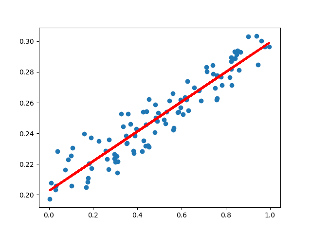
# 展示拟合结果
y_pred = model.predict(x_train)
plt.scatter(x_train, y_train)
plt.plot(x_train, y_pred, "r-", lw=3)
plt.show()#结果展示
#非线性回归
#示例程序
import numpy as np
import matplotlib.pyplot as plt
from keras.src.models import Sequential # Keras 中的顺序模型
from keras.src.layers import Input, Dense, Activation # Keras 中的全连接层和激活函数
from keras.src.optimizers import SGD # Keras 中的 SGD 优化器
# 构造训练样本
x_train = np.linspace(-0.5, 0.5, 200) # 一维数据,样本量 200,等差线性分布
noise = np.random.normal(0, 0.02, x_train.shape) # 噪声数据,服从高斯分布(正态分布)
y_train = np.square(x_train) + noise
# 编译模型
model = Sequential() # 顺序模型
model.add(Input(shape=(1,)))
model.add(Dense(units=5)) # 全连接层,输出数据 10 维, 输入数据 1 维
model.add(Activation("tanh")) # tanh 激活函数
model.add(Dense(units=1)) # 全连接层,输出数据 1 维, 输入数据 10 维
model.add(Activation("tanh")) # tanh 激活函数
sgd = SGD(learning_rate=0.2) # 设置随机梯度下降算法的学习率
model.compile(optimizer=sgd, loss="mse") # 优化算法:随机梯度下降,损失函数:均方差
# 训练样本
for step in range(5000):
cost = model.train_on_batch(x_train, y_train)
if step % 500 == 0:
print("cost: ", cost)
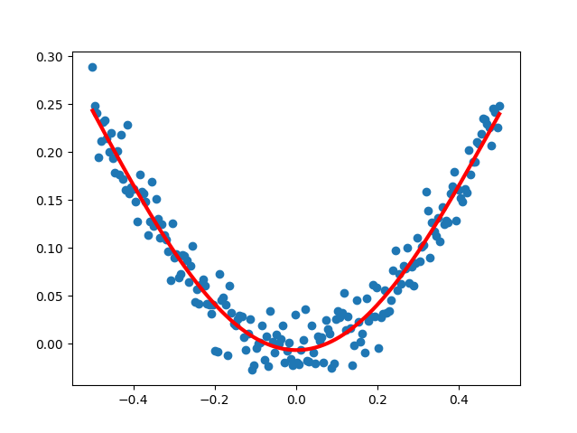
# 展示拟合结果
y_pred = model.predict(x_train)
plt.scatter(x_train, y_train)
plt.plot(x_train, y_pred, "r-", lw=3)
plt.show()#结果展示
#MNIST 数据分类
#示例程序
from keras.src.datasets import mnist
from tensorflow.python.keras.utils import np_utils
from keras.src.models import Sequential
from keras.src.layers import Input, Dense, Dropout
from keras.src.optimizers import SGD

# 载入数据集(第一次运行会联网下载)
(x_train, y_train), (x_test, y_test) = mnist.load_data()
print("x_train: ", x_train.shape, "y_train: ", y_train.shape)
print("x_test:  ", x_test.shape, "y_test:  ", y_test.shape)
x_train = x_train.reshape(x_train.shape[0], -1) / 255.0  # 归一化
x_test = x_test.reshape(x_test.shape[0], -1) / 255.0 # 标签值转为 one-hot 码
y_train = np_utils.to_categorical(y_train, num_classes=10)
y_test = np_utils.to_categorical(y_test, num_classes=10)

# 编译模型
model = Sequential()  # 顺序模型
model.add(Input(shape=(x_train.shape[1],)))
# 全连接层(隐藏层),输出数据 200 维,输入数据维度由训练数据本身决定, 使用 tanh 激活函数
model.add(Dense(units=196, input_dim=x_train.shape[1], activation="relu"))
# 全连接层(隐藏层),输出数据 100 维,输入数据由前一层决定, 使用 tanh 激活函数
model.add(Dense(units=98, activation="relu"))
model.add(Dropout(0.4))  # 让 20% 的神经元不工作(防止过拟合的一种手段)
# 全连接层(输出层),输出数据 10 维(共 10 种手写数字),输入数据由前一层决定, 使用 softmax 激活函数
model.add(Dense(units=10, activation="softmax"))
sgd = SGD(learning_rate=0.1)  # 设置随机梯度下降算法的学习率
model.compile(
    optimizer=sgd,
    loss="categorical_crossentropy",
    metrics=["accuracy"])  # 优化算法:随机梯度下降,损失函数:交叉熵

# 训练样本
model.fit(x_train, y_train, batch_size=32, epochs=10)

# 评估模型
loss, accuracy = model.evaluate(x_test, y_test)
print("loss= ", loss, "accuracy= ", accuracy)